5 LAB VI: Inference for numerical data (2 samples)

When we have finished this Lab, we should be able to:

Learning objectives

Applying hypothesis testing
Compare two independent samples
Compare paired (related) samples
Interpret the results

5.1 Two-sample t-test (Student’s t-test)

Two sample t-test (Student’s t-test) can be used if we have two independent (unrelated) groups (e.g., males-females, treatment-non treatment) and one quantitative variable of interest.

5.1.1 Opening the file

Open the dataset named depression from the file tab in the menu:

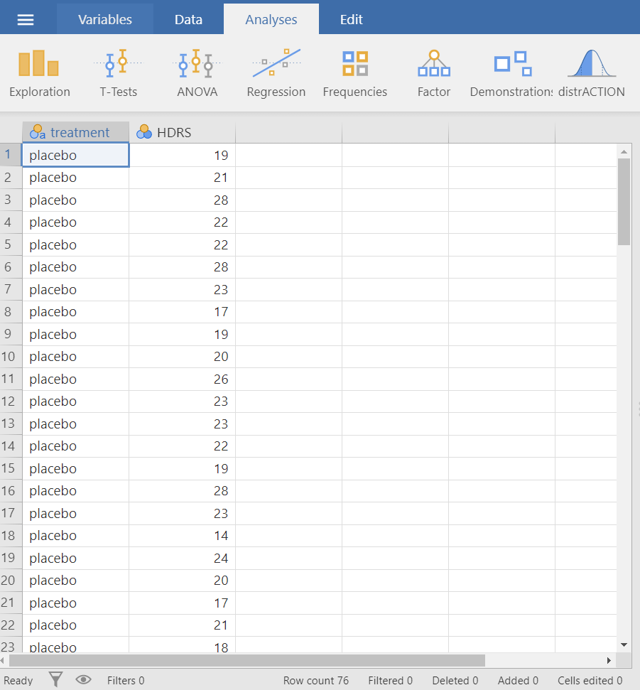
The dataset depression includes 76 patients and has two variables. The treatment variable and the HDRS variable (Figure 5.1). Double-click on the variable name HDRS and change the measure type from nominal to continuous .

5.1.2 Research question

In an experiment designed to test the effectiveness of paroxetine for treating bipolar depression, the participants were randomly assigned into two groups (intervention Vs placebo).

The researchers used the Hamilton Depression Rating Scale (HDRS) to measure the depression state of the participants and wanted to find out if the HDRS score is different in paroxetine group as compared to placebo group at the end of the experiment. The significance level α was set to 0.05.

Note A score of 0–7 in HDRS is generally accepted to be within the normal range, while a score of 20 or higher indicates at least moderate severity.

5.1.3 Hypothesis Testsing for the Student’s t-test

Null hypothesis and alternative hypothesis

$H_{0}$ : the means of HDRS in the two groups are equal ( $μ_{1} = μ_{2}$ )
$H_{1}$ : the means of HDRS in the two groups are not equal ( $μ_{1} \neq μ_{2}$ )

5.1.4 Assumptions

Check if the following assumptions are satisfied

The data are normally distributed in both groups
The data in both groups have similar variance (also named as homogeneity of variance or homoscedasticity)

A. Explore the descriptive characteristics of distribution for each group and check for normality

The distributions can be explored visually with appropriate plots. Additionally, summary statistics and significance tests to check for normality (e.g., Shapiro-Wilk test) and for equality of variances (e.g., Levene’s test) can be used.

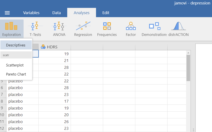
On the Jamovi top menu navigate to

as shown below in Figure 5.2.

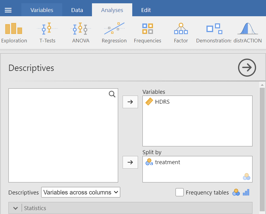
Figure 5.2: In the Analyses Tab select Exploration and click on Descriptives.

The Descriptives dialogue box opens. Drag the variable HDRS into the Variables box and split it by the treatment variable, as shown below (Figure 5.3):

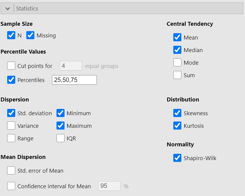
Figure 5.3: Split the variable HDRS by treatment group

We can now select the relevant descriptive statistics such as Percantiles, Skewness, Kurtosis and the Shapiro-Wilk test from the Statistics section:

Figure 5.4: In the Statistics section select the descriptive statistics of interest.

Once we have selected our descriptive statistics, a table will appear in the output window on our right-hand side, as shown below:

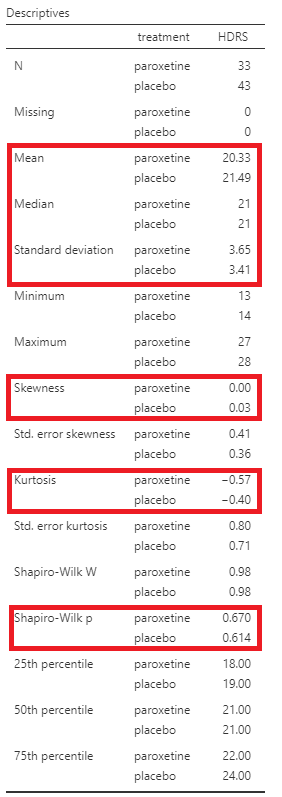
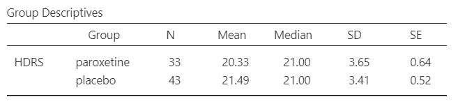
Figure 5.5: Descriptive statistics of HDSR by treatment group

The means are close to medians (20.3 vs 21 and 21.5 vs 21). The skewness is approximately zero (symmetric distribution) and the (excess) kurtosis is close to zero (mesokurtic distribution) indicating normal distributions for both groups.

Additionally, the Shapiro-Wilk tests of normality suggest that the data for the HDRS in both groups, paroxetine and placebo, are normally distributed (p=0.67 >0.05 and p=0.61 >0.05, respectively). (NOTE: If the $p \geq 0.05$ , then the data came from a normally distributed population).

Remember: Hypothesis testing for Shapiro-Wilk test for normality

$H_{0}$ : the data came from a normally distributed population.

$H_{1}$ : the data tested are not normally distributed.

If p − value < 0.05, reject the null hypothesis, $H_{0}$ .
If p − value ≥ 0.05, do not reject the null hypothesis, $H_{0}$ .

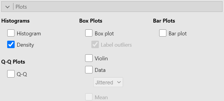
Then we can check the Density from Histograms in the Plot section, as shown below (Figure 5.7):

Figure 5.6: In the Plot section select Density from Histograms.

A graph is generated in the output window on our right-hand side, as shown below:

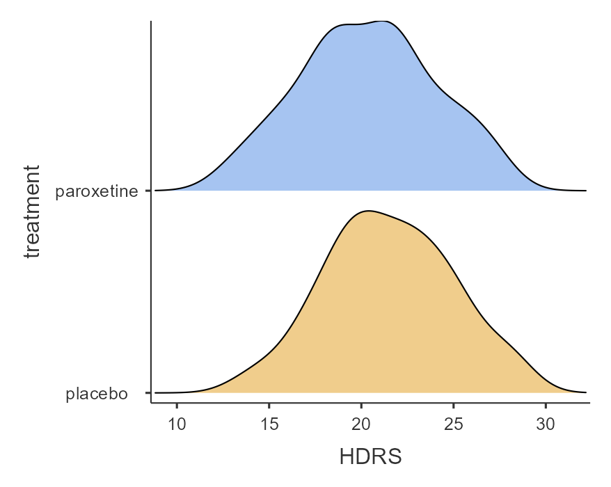
Figure 5.7: In the Plots section select Density from Histograms.

The above figure shows that the data are close to symmetry and the assumption of a normal distribution is reasonable.

B. Homogeneity of variance

The second assumption that should be satisfied is the homogeneity of variance. We observe in the summary table of Figure 5.5 that the two standard deviations (3.65 vs 3.41) are similar (see also below the Levene’s test for equality of variances in Figure 5.11).

5.1.5 Run the Student’s t-test

Perform a Student’s t-test

We will perform a Student’s t-test to test the null hypothesis that the mean HDRS score is the same for both groups (paroxetine and placebo).

We select:

Figure 5.8: Conducting an Independent Samples T-Test.

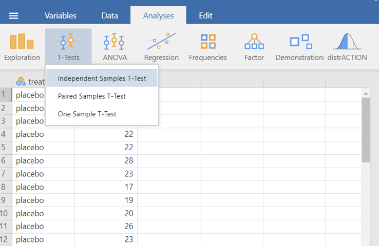
The Independent Samples T-Test dialogue box opens. Drag and drop the numeric variable HSDR to Dependent Variables and the independent variable treatment to Grouping Variable, as shown below Figure 5.9:

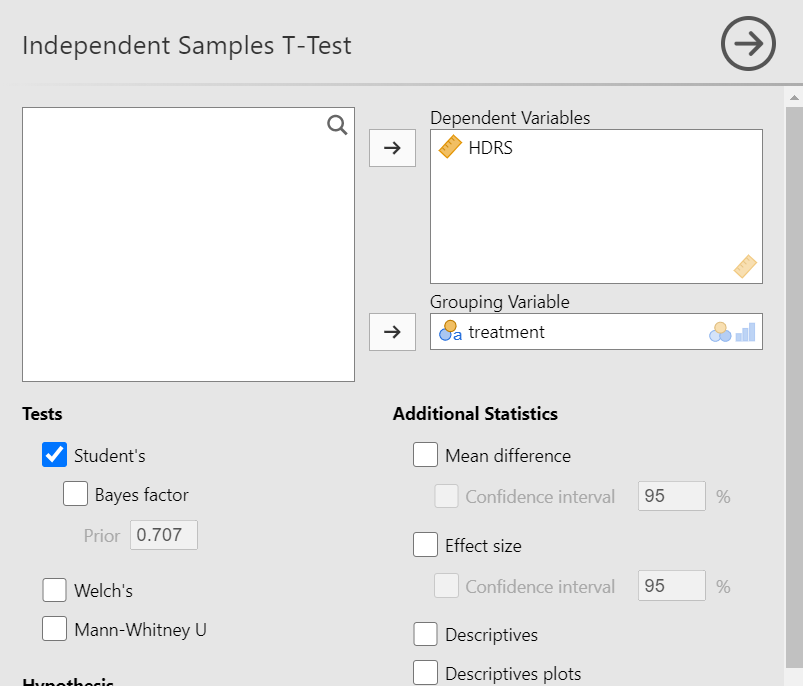
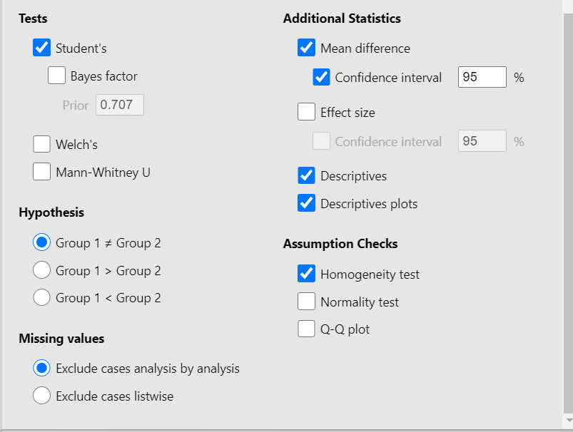
Figure 5.9: The Independent Samples T-Test dialogue box

We observe that we can select between the following three Tests: Students’s (the default), Welch’s, or Mann-Whitney U. At the moment, we keep the default choice of Students’s test. From Additional Statistics check the Mean difference, Confidence Intervals, Descriptive, and Descriptive plots boxes. Finally, from Assumption Checks tick the Homogeneity test. We will end up with the following screen:

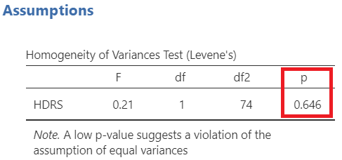
Figure 5.10: Additional statistics and tests.

First, we look at the table of Levene's test for equality of variances (Figure 5.11):

Remember: Hypothesis testing for Levene’s test for equality of variances

$H_{0}$ : the variances of HDRs in two groups are equal

$H_{1}$ : the variances of HDRs in two groups are not equal

If p − value < 0.05, reject the null hypothesis, $H_{0}$ .
If p − value ≥ 0.05, do not reject the null hypothesis, $H_{0}$ .

Since p = 0.646 > 0.05, the $H_{0}$ of the Levene’s test is not rejected and we keep the default choice of Students’s test (Figure 5.10). (NOTE: If the $p \geq 0.05$ , then the population variances of HDRS in two groups groups are assumed equal).

If the assumption of equal variances is not satisfied (Levene’s test gives p < 0.05, reject $H_{0}$ ), the Welch’s test should be used from the available Tests in Jamovi (Figure 5.10).

Next, we can inspect again the results in the group descriptives table (Figure 5.12) and pertinent plots (Figure 5.13):

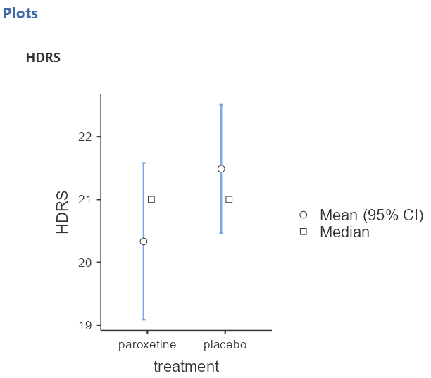
Figure 5.13: Plot of mean (95% CI) and median of HDRS by treatment.

Finally, we present the results of the Student’s t-test in the table of the Figure 5.14:

Figure 5.14: The results of the Student’s t-test.

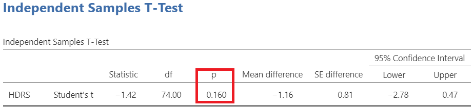
The p-value = 0.16 is greater than 0.05. There is no evidence of a significant difference in mean HDRS between the two groups (failed to reject $H_{0}$ ). The difference between means (20.33 - 21.49) equals to -1.16 units of the HDRS and note that the 95% confidence interval of the difference in means (-2.78 to 0.47) includes the hypothesized null value of 0. Based on these results, there is not evidence that paroxetine is effective as a treatment for bipolar depression.

Note that the paroxetine sample (n= 33) has 32 (33-1) degrees of freedom and the placebo sample (n= 43) has 42 (43-1), so we have 74 (32 + 42) df in total. Another way of thinking of this is that the complete sample size is 76, and we have estimated two parameters from the data (the two means), so we have 76-2 = 74 df.

The Student t-test for two independent samples does not have any restrictions on $n_{1}$ and $n_{2}$ —they can be equal or unequal. However, equal samples are preferred because when a total of 2n subjects are available, their equal division among the groups maximizes the power to detect a specified difference.

Mann-Whitney U test

When there is violation of normality, the Mann-Whitney U test can be selected from the available Tests in Jamovi (Figure 5.11). This test compares two independent samples based on the ranks of the values and is often considered the non-parametric equivalent to the Student’s t-test.

5.2 Paired samples t-test

The paired samples design can effectively reduce the effect of non-treatment factors and improve the efficiency of the experiment. A paired samples t-test is used to estimate whether the means of two related measurements are significantly different from one another.

Open the dataset named weight from the file tab in the menu:

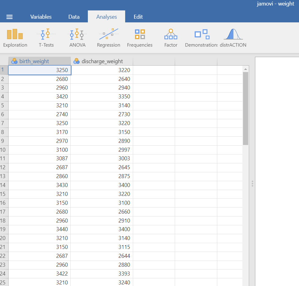
The dataset weight contains the birth and discharge weight of 25 newborns (Figure 5.15). Double-click on the name of the variables birth_weight and discharge_weight to change the measure type from nominal to continuous .

5.2.1 Research question

We might ask if the mean difference of the weight in birth and in discharge equals to zero or not. If the differences between the pairs of measurements are normally distributed, a paired t-test is the most appropriate statistical test.

5.2.2 Hypothesis Testsing for the paired samples t-test

Null hypothesis and alternative hypothesis

H₀: the mean difference in weight is zero ( $μ_{d} = 0$ )
H₁: the mean difference in weight is non-zero ( $μ_{d} \neq 0$ )

5.2.3 Assumptions

Check if the following assumption is satisfied

The differences between the pairs of measurements, $d_{i}$ s, are normally distributed. (NOTE: It is not essential for the original observations to be normally distributed).

Explore the characteristics of the distribution of differences, $d_{i}$

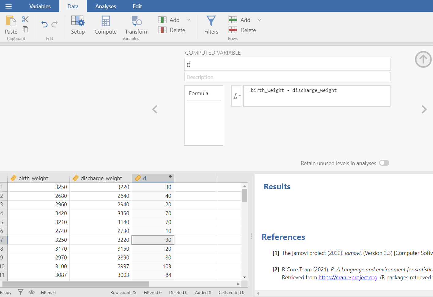
First, we have to calculate the differences $d_{i} = b i r t h_w e i g h t_{i} - d i s c h a r g e_w e i g h t_{i}$ (Figure 5.16) from Data tab in the main menu of Jamovi. For more details go to the section 11.6 Transforming data: Computing a new variable in Chapter 3.

Figure 5.16: Calculation of the variable of differences d

The distributions of the differences, $d_{i}$ , can be explored with appropriate plots and summary statistics.

On the Jamovi top menu navigate to

as shown below in Figure 5.17.

Figure 5.17: In the Analyses Tab select Exploration and click on Descriptives.

The Descriptives dialogue box opens. Drag the variable d into the Variables box, as shown below (Figure 5.18):

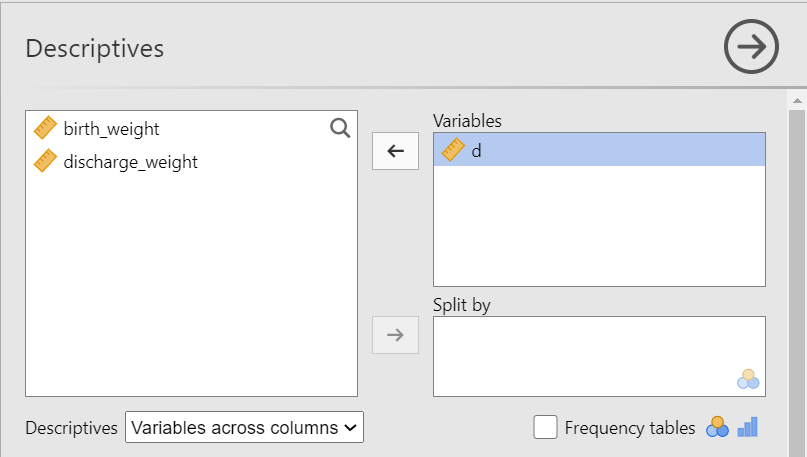
Figure 5.18: Drag the variable of the differences `d` into the `Variables` box

We can now select the relevant descriptive statistics such as Percantiles, Skewness, Kurtosis and the Shapiro-Wilk test from the Statistics section:

In the Statistics section select the descriptive statistics of interest.

Once we have selected our descriptive statistics, a table will appear in the output window on our right-hand side, as shown below:

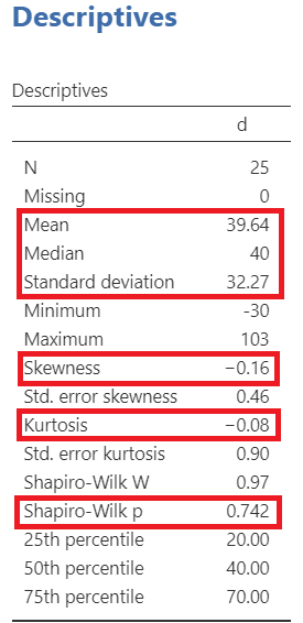
Figure 5.19: Descriptive statistics of the differences.

The mean is close to median (39.6 vs 40). Moreover, both skewness and (excess) kurtosis are approximately zero indicating a symmetric and mesokurtic distribution of the weight differences.

Then we can check the Density from Histograms in the Plot section, as shown below (Figure 6.6):

In the Plot section select Density from Histograms.

A graph is generated in the output window on our right-hand side, as shown below:

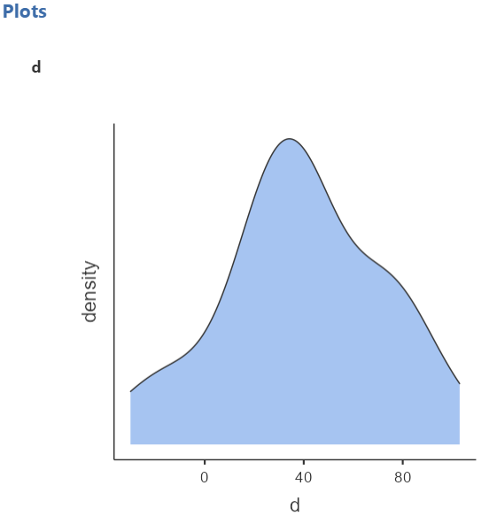
Figure 5.20: In the Plots section select Density from Histograms.

The above figure shows that the data are close to symmetry and the assumption of a normal distribution is reasonable.

Additionally, the Shapiro-Wilk test of normality suggests that the data for the differences, $d_{i}$ , are normally distributed (p=0.74 >0.05). (NOTE: If the $p \geq 0.05$ , then the data came from a normally distributed population).

5.2.4 Run the paired samples t-test

Perform a paired samples t-test

We will perform a paired samples t-test to test the null hypothesis that the mean difference in weight is zero.

We select:

Figure 5.21: Conducting a Paired Samples T-Test.

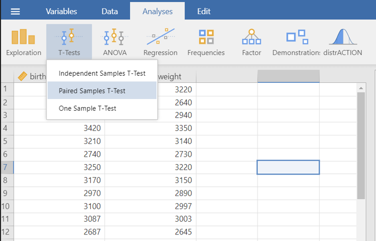
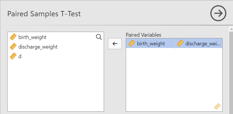
The Paired Samples T-Test dialogue box opens. Drag and drop the variables birth_weight and discharge_weight to Paired Variables, as shown below Figure 5.22:

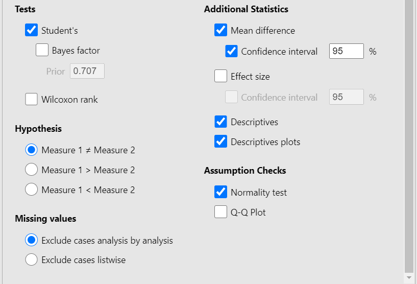
Figure 5.22: The Paired Samples T-Test dialogue box

We observe that we can select between the following two Tests: Students’s or Wilcoxon rank. We keep the default choice of Students’s paired t-test. Moreover, from Additional Statistics check the Mean difference, Confidence Intervals, Descriptive, and Descriptive plots boxes. Finally, from Assumption Checks tick the Normality test. We will end up with the following screen:

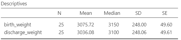
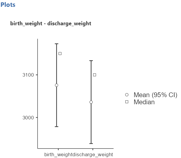
Figure 5.23: Additional statistics and tests.

Next, we can inspect the results in the table with descriptive statistics (Figure 5.24) and plots (Figure 5.13):

Figure 5.24: Table with descriptive statistics.

Figure 5.25: Plot of mean and median of *birth weigt* and *discharge_weight*.

The Shapiro-Wilk test of normality of the differences has previously calculated (Figure 5.19) and is also presented below:

Figure 5.26: Test of normality of the differences.

Finally, we present the results of the Student’s paired samples t-test in the table of the Figure 5.27:

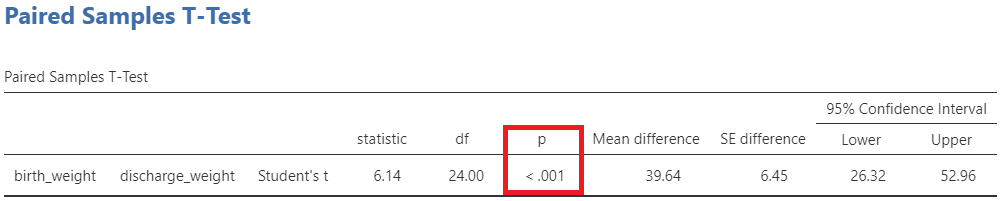
Figure 5.27: The results of the Paired Samples t-test.

There was a significant reduction in weight (39.6 g) after the discharge (p-value <0.001 that is lower than 0.05; reject $H_{0}$ ). Note that the 95% confidence interval (26.3 to 52.9) doesn’t include the null hypothesized value of 0. However, is this reduction of clinical importance?

Wilcoxon Signed-Rank test

When there is violation of normality, the Wilcoxon Rank test can be selected from the available Tests in Jamovi (Figure 5.23). This test is based on the sign and the magnitude of the rank of the differences between pairs of measurements, rather than the actual values. It is often considered the non-parametric equivalent to the Student’s paired samples t-test.