3 LAB I: Introduction to Jamovi and data preparation – Basic Statistics for the Social Sciences

3.1 Why Jamovi?

Jamovi is a new fee open “3rd generation” statistical software that is built on top of the programming language R (Figure 3.1). Designed from the ground up to be easy to use, Jamovi is a compelling alternative to costly statistical products such as SPSS and SAS.

Figure 3.1: Jamovi is free and open statistical software

Some other advantages are:

User-friendly point-and-click interface.
Displays informative tables and clear visuals.
Supports add-on modules for advanced statistical analysis.
Allows integration with R.
Provides access to a user guide and community resources on the Jamovi website.

3.2 Downloading and installing Jamovi

Jamovi is available for Windows (64-bit), macOS, Linux and ChromeOS. Installation on desktop is quite straight-forward. Just go to the Jamovi download page https://www.jamovi.org/download.html, and download the latest version (current release) for your operating system.

3.3 Navigating Jamovi

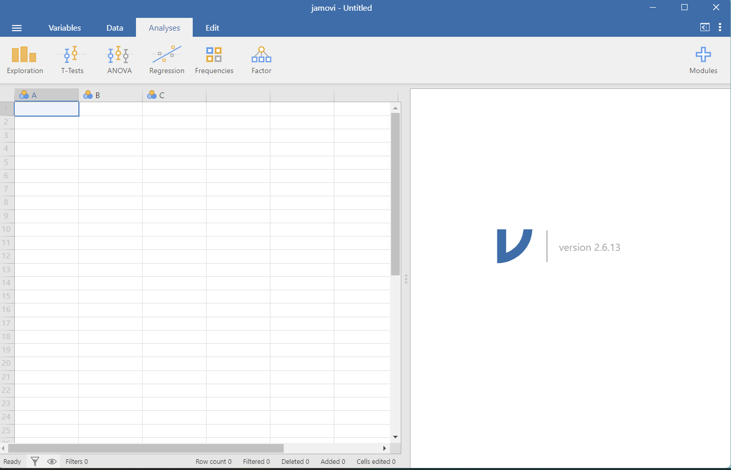
When jamovi first opens, we will see a screen something like in Figure 3.2.

To the left is the spreadsheet view, and to the right is where the results of statistical tests appear. Down the middle is a bar separating these two regions, and this can be dragged to the left or the right to change their sizes.

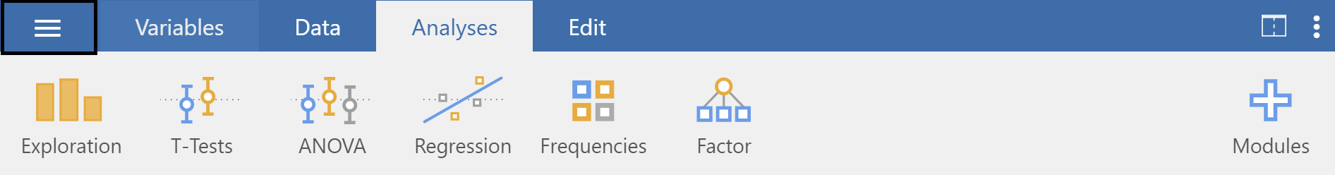
Let’s take a quick look at the Jamovi Main Menu, referred to hereafter as the Menu, as shown in Figure 3.3. This Menu is displayed at the very top of the Jamovi screen:

Figure 3.3: The menu bar provides access to all functions of the program.

There are six tabs in the Menu (from left to right): 1. File (a layer with three horizontal levels $\equiv$), 2. Variables, 3. Data, 4. Analyses, 5. Edit, and 6. Settings (the three dots $\vdots$ at the top right of the window) tabs. A toolbar appears whenever we click on a Menu tab (Table 3.1).

Menu tab	Toolbar
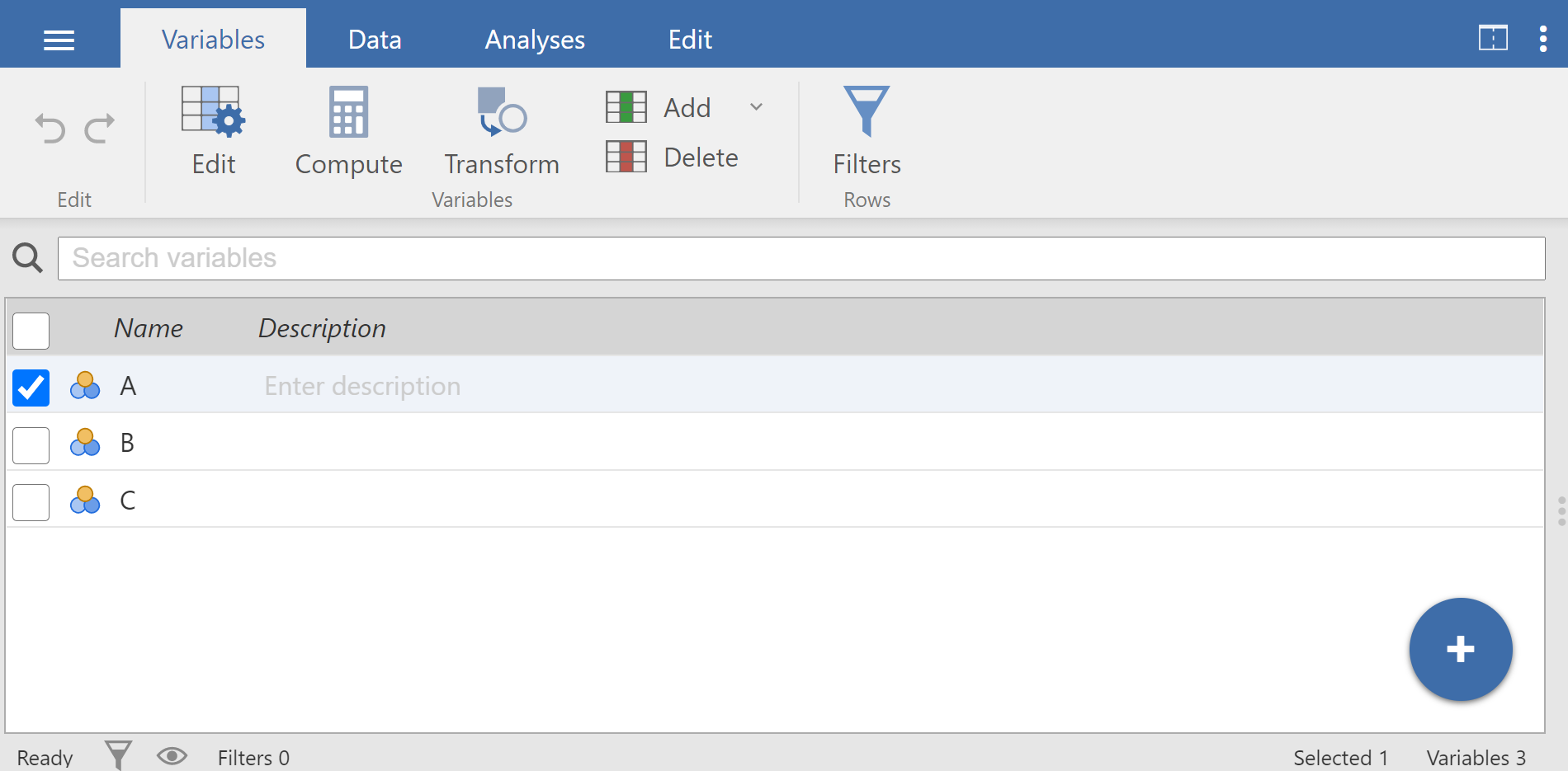
File tab (\(\equiv\)) The file tab allows us to open/import existing files, save and export our files.
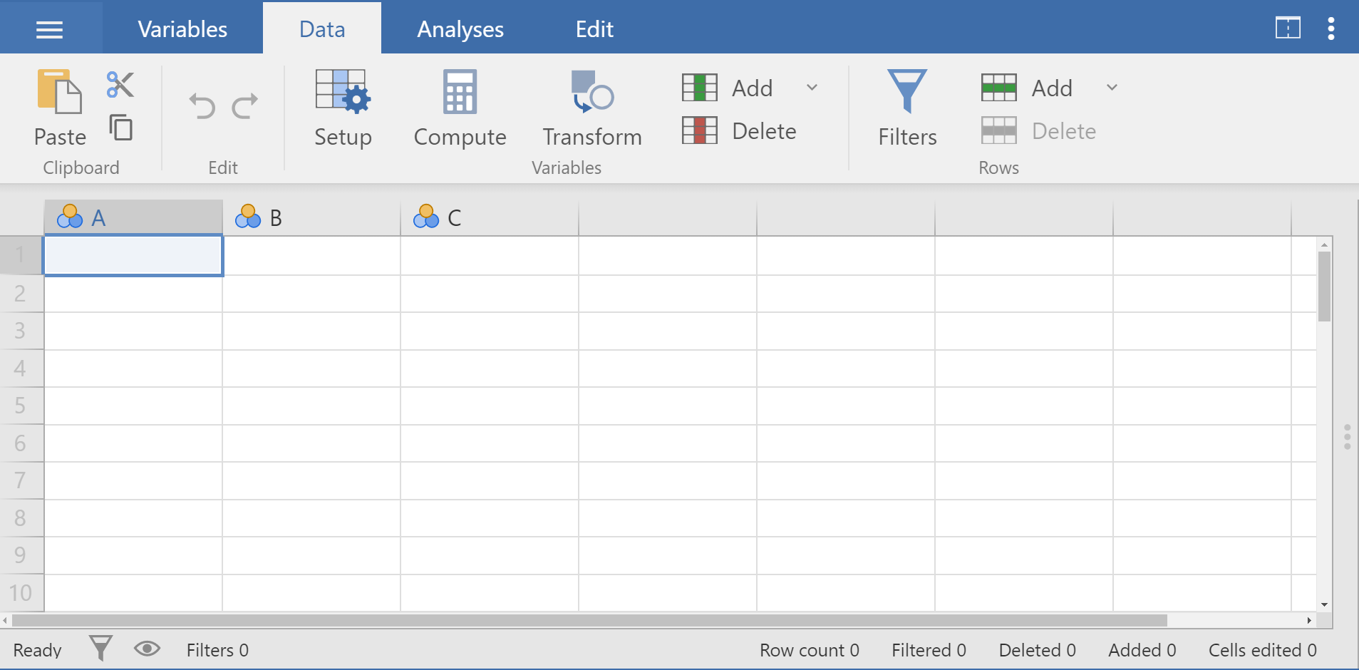
Variables tab This allows us to view and search our variables in a list view.	This view allows us to easily navigate our variables and do the following: Search for a variable by scrolling through the list or search for one by name. Edit the variable names and descriptions by double-clicking in the relevant field. Edit our variable details by double-clicking on the data symbol (the screen will appear for us to add all the necessary information). Create a new variable by clicking on the in the bottom right corner. \|
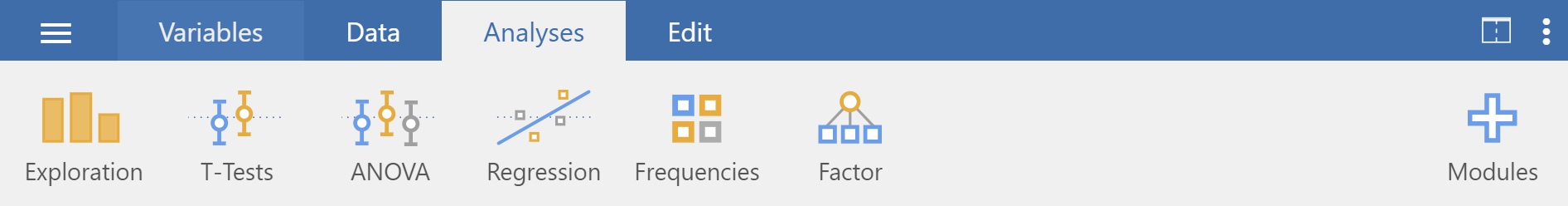
Data tab Here we will see our raw data which are organised like Excel in rows and columns. We can also manipulate our data and add new variables when necessary.	Specifically, this tab allows us to do the following: Rename and add details to existing variables. Click on the Setup button, or double-click on the variable we want to manage. Compute and transform variables Add and/or Delete variables (columns) Add Filters Add and/or Delete Rows
Analyses tab It includes the available statistical analyses that can be performed by Jamovi.	We will spend most of our time in the Analyses Tab. The following six modules are pre-installed: Exploration T-Tests ANOVA Regression Frequencies Factor For example, if we want to perform regression analysis, we simply click the ’’Regression” button. All other modules need to be installed using the Modules button (Plus button) in our top-right \|
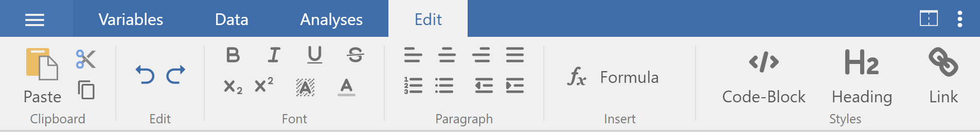
Edit tab It includes a toolbar similar to a word processor.	We can add extra information to our results using the buttons that are very similar to what we would find in Word (though there are fewer options).
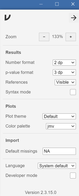
Settings tab (the three dots \({\vdots}\) at the top right of the window) It includes the application settings that can be manged by the users according to their preferences.	We can apply our preferences for a number of settings such as: How many decimal numbers we want. If we want to learn R, we can also display the R syntax. Our graph color scheme. Our default missing value.

3.4 Types of Variables in Jamovi

Data variables can be one of four measure types:

Nominal: This type is for nominal categorical variables.
Ordinal: This type is for ordinal categorical variables.
Continuous : this type is for variables with numeric values which are considered to be of Interval or Ratio scales.
ID: This will usally be our first column. This can be text or numbers, but it should be unique to each row.

Additionally, data variables can be one of three data types:

Integer: These are full numbers e.g. 1, 2, 3, … 100, etc. - Integers can be used for all three measure types . When used for Nominal/Ordinal data numbers will represent labels e.g. male=1; female=2.
Decimal: These are numbers with decimal points. e.g. 1.3, 5.6, 7.8, etc. - This will usually only be used for continuous data.
Text: This can be used for ordinal and nominal data.

The measure types are designated by the symbol in the header of the variable’s column. Note that some combinations of data-type and measure-type don’t make sense, and Jamovi won’t let us choose these.

Table 3.2: Types of data and measures

		Measure
Data	Nominal	Ordinal	Continuous
Integer	${\checkmark}$	${\checkmark}$	${\checkmark}$
Decimal			${\checkmark}$
Text	${\checkmark}$	${\checkmark}$

3.5 Importing data

3.5.1 The dataset

It is possible to simply begin typing values into the Jamovi spreadsheet as we would with any other spreadsheet software. Alternatively, existing datasets in a range of formats (OMV, Excel, CSV, SPSS, R data, Stata, SAS) can be opened in Jamovi. We will use the following dataset as an example (Figure 9.1).

Figure 3.4: Table with raw data.

(NOTE: You can find other formats of the data (OMV, Excel) at the link: https://osf.io/gvctz/).

The meta-data (data about the data) for this dataset are as following:

sex: sex (1 = male, 2 = female).
age: age in years.
time_spend: hours spent on social media.
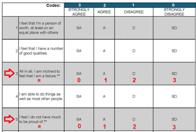
$q_1 ... q_{10}$: Ten questions (items) of Rosenberg Self-Esteem Scale (RSES). The 10 items are answered on a four point scale ranging from strongly agree to strongly disagree coded as follows: Strongly Agree = 3, Agree = 2, Disagree = 1, and Strongly Disagree = 0.

Positively worded Items 1, 2, 4, 6, and 7.
Negatively worded Items 3, 5, 8, 9, and 10 (codes should be reversed).

Figure 3.5: Codes should be reversed for the negatively worded Items.

The scale ranges from 0-30 (we add the scores for all items), with 30 indicating the highest total score possible.

More information for the RSES: Rosenberg Self-Esteem Scale.

3.5.2 Opening the file

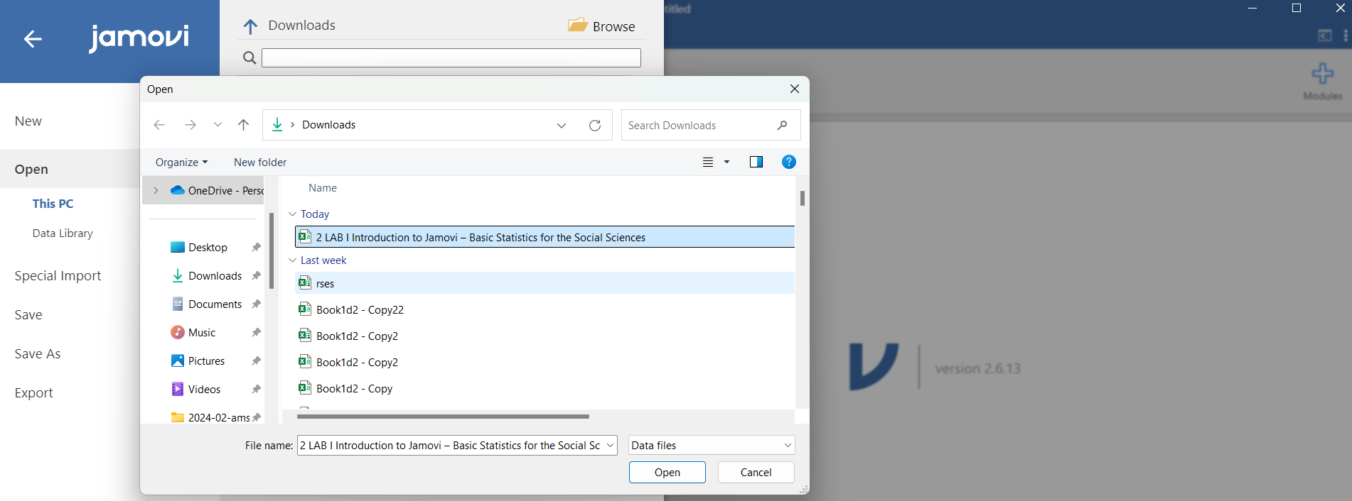
To open this csv file, click on the File tab at the top left hand corner (just left of the Variables tab) (Figure 3.6).

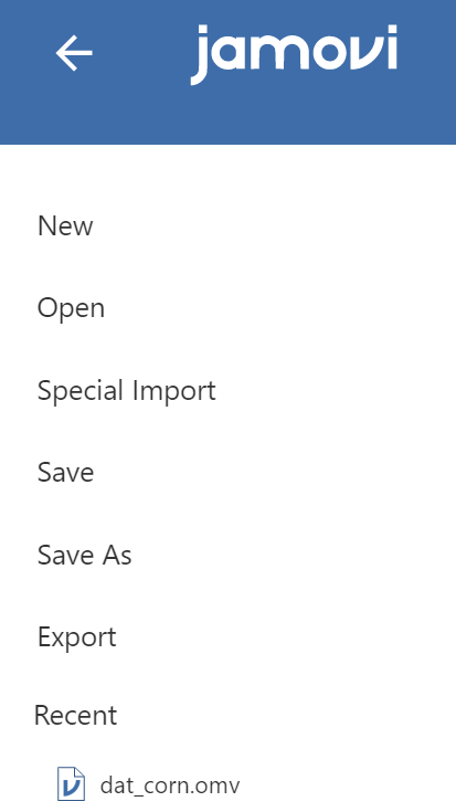
This will open the menu shown in Figure 3.7. Select ‘Open’ and then ‘This PC’. Choose the downloaded file from the files listed on ‘Browse’ which are stored on our computer folders:

Figure 3.7: Open an existing file stored on our computer into Jamovi.

The flowchart of the process is:

flowchart LR
  A(File tab) -.-> B(Open) -.-> C(This PC) -.-> D(Browse) -.-> E(Open \n 'the downloaded file')

We should see data now in the Spreadsheet view (Figure 3.8).

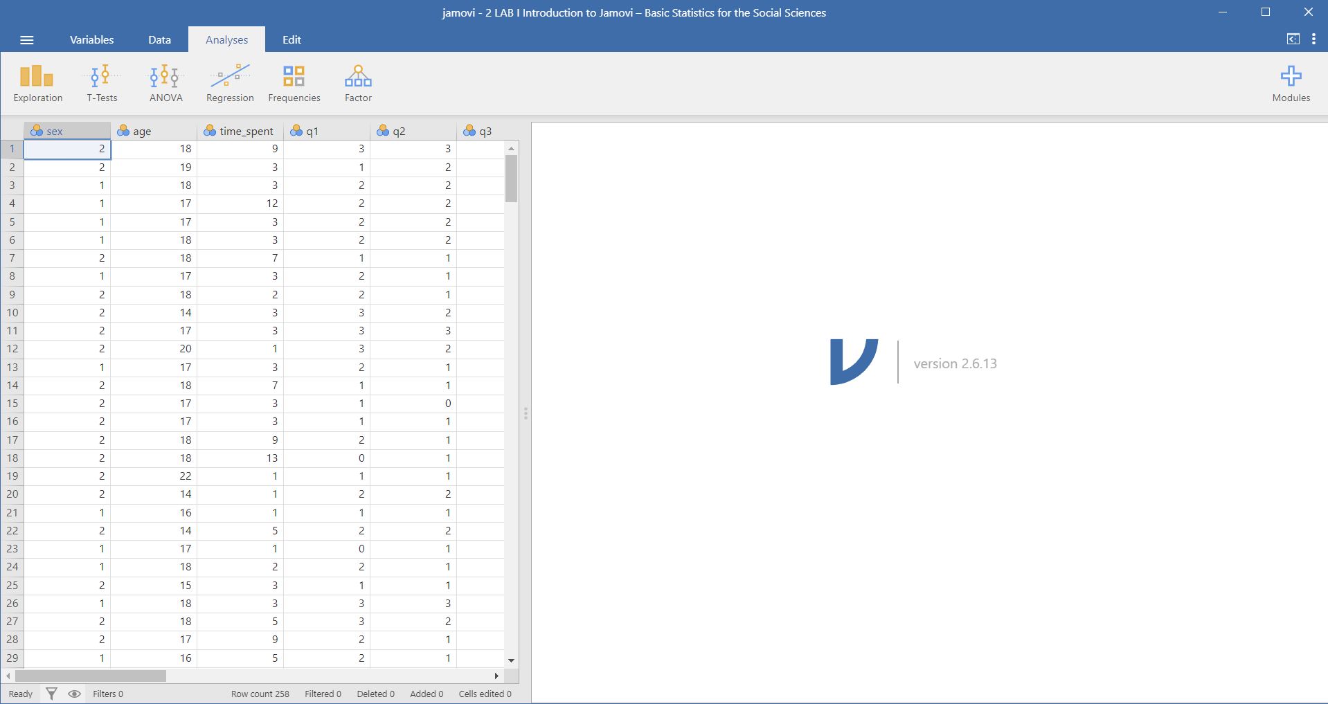
As we can see this is a data set with 258 observations and 13 variables. JAMOVI has classified all the variables as nominal ; however, only the sex variable is actually nominal.

3.6 Adding labels to codes

sex variable

The first variable, named sex, is a categorical variable coded as 1 for males and 2 for females. Notice that it is correctly identified as a nominal variable in Jamovi.

We can assign labels to numerically coded values of categorical variables, such as sex, by accessing the data variable settings. One way to achieve this is by double-clicking on the variable name sex, which opens the additional menu of variable settings at the top of the Jamovi screen (Figure 3.9).

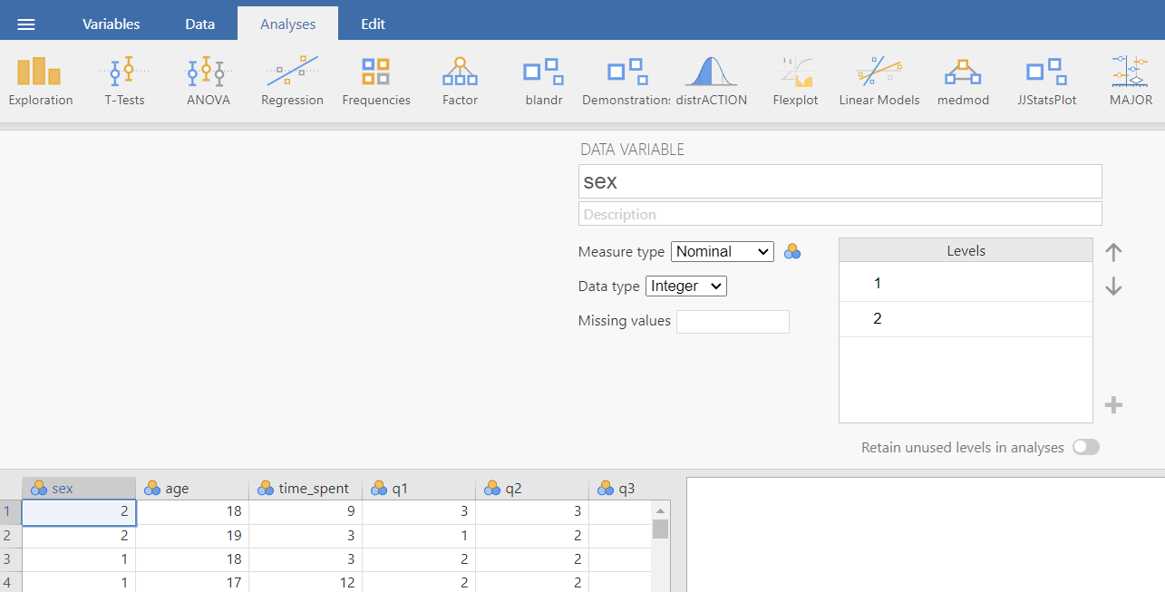
Figure 3.9: An additional menu appears at the top of the Jamovi screen after double-clicking on the variable name sex.

In this menu, we will find the Levels setup. Here, we can specify the labels that should appear for each category level. Click on the number “1” in the Levels box to edit its label, changing it from “1” to “male”. Similarly, click on the number “2” and change it to “female” (Figure 3.10).

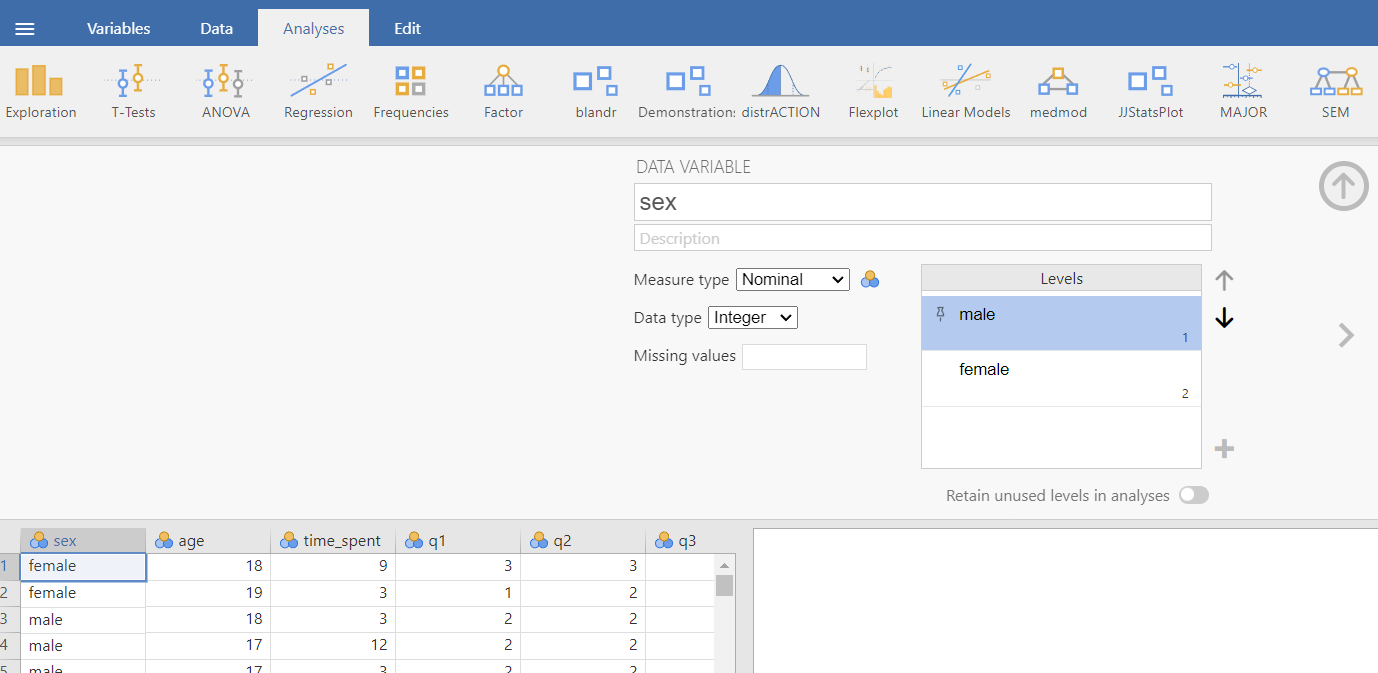
Figure 3.10: Adding labels to numerically coded Values.

Notice how the numbers “1” and “2” have moved to the lower right under the text we’re typing, allowing us to still see which label corresponds to each numerical code. Press Enter or click anywhere outside the labels box to save these labels.

We close the variable settings by pressing the arrow in the top-right corner .

3.7 Changing the measure type

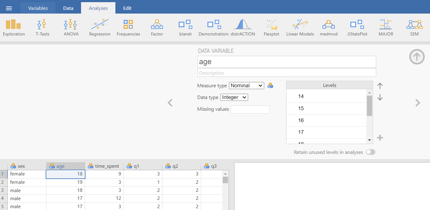
Next, we will change the measure type of age and time_spent variables from nominal to continuous.

age variable

Double-click on the variable name age to open the data variable settings, as shown in Figure 3.11:

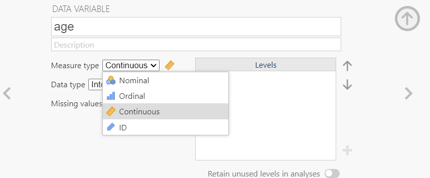
Figure 3.11: Data variable menu settings for the age variable.

From the drop-down list of “Measure type” we select the continuous type , as shown in Figure 3.12.

Figure 3.12: Change the measure type of age from nominal to continuous. .

time_spent variable

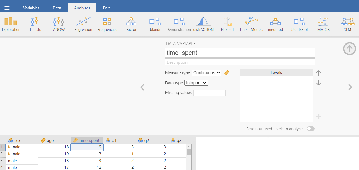
Instead of closing the data variable menu using the arrow in the top-right corner, we can click on the to proceed to the next variable setting, time_spent. As before, we select the continuous type for this variable from the “Measure type” drop-down list, as shown in Figure 3.13.

Figure 3.13: Change the measure type of time_spent from nominal to continuous.

We close the variable settings by pressing the arrow in the top-right corner .

q1 to q10 variables

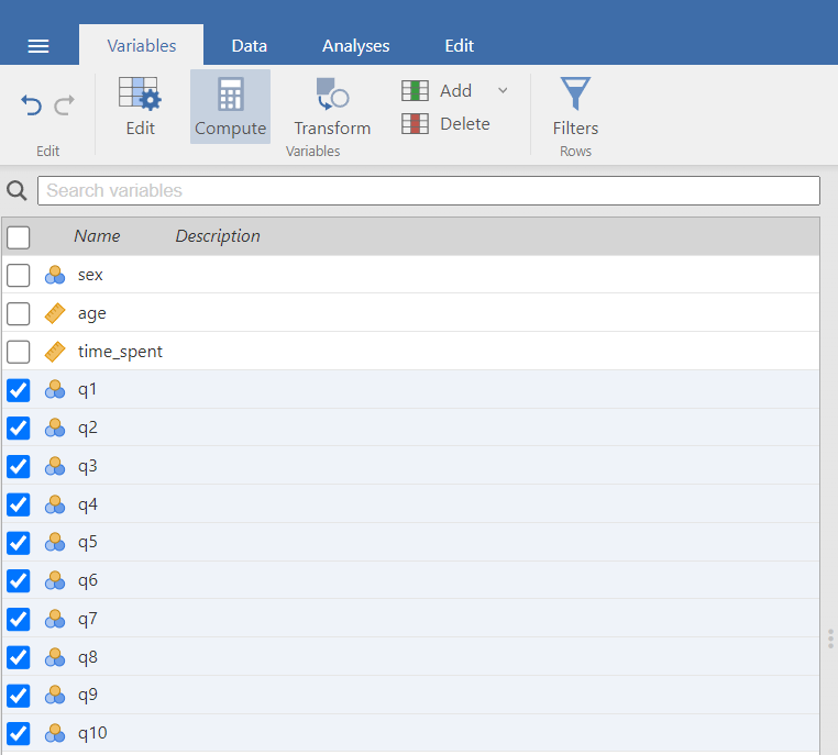
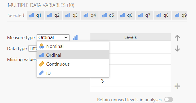
Finally, we will change the measure type of q1 to q10 variables from nominal to ordinal. In the Variables tab, we select the checkboxes for the q1 through q10 variables, as shown in Figure 3.14.

Figure 3.14: Change the measure type of time_spent from nominal to continuous.

After that, we click on the Edit button to open the data variable settings, as shown in Figure 3.15.

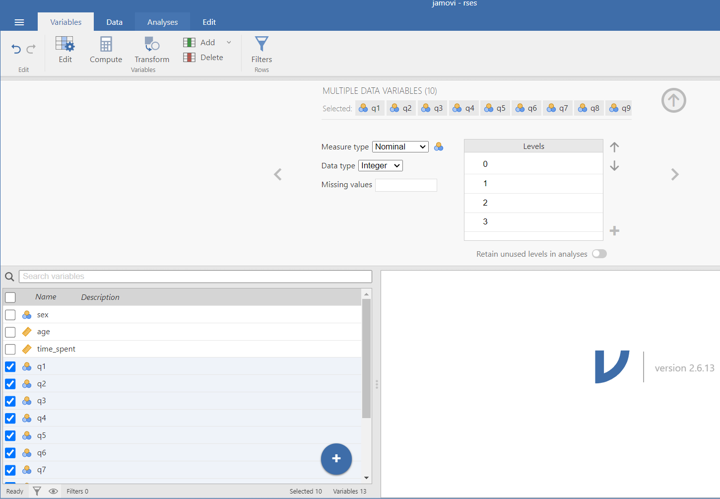
Figure 3.15: Change the measure type of time_spent from nominal to continuous.

From the drop-down list of “Measure type” we select the ordinal type , as shown in Figure 3.16.

Figure 3.16: Change the measure type of q1 to q10 from nominal to ordinal.

3.8 Filtering rows

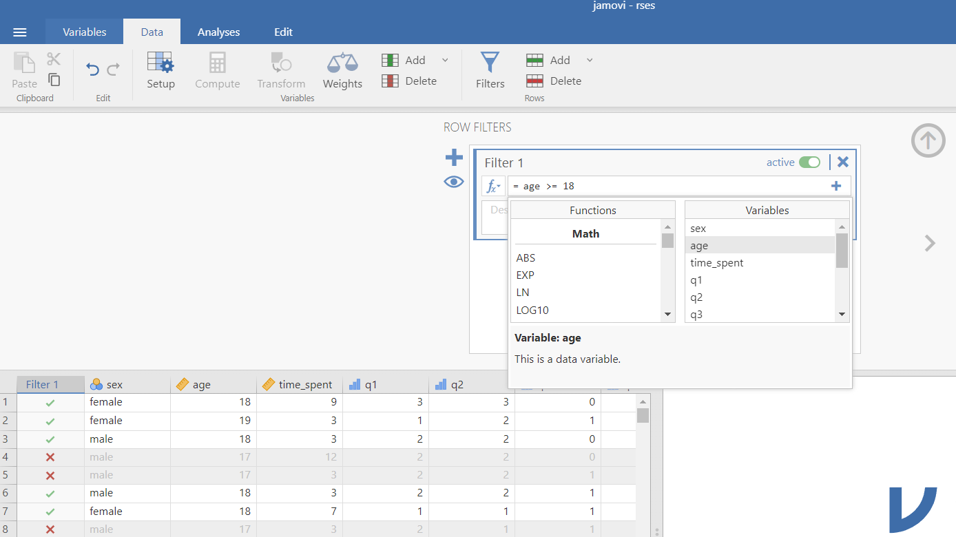
Next, we select the Filters button from the Data tab. This opens the “Row FILTERS” view at the top of the Jamovi screen where we can add a filter called “Filter 1” (Figure 3.17). Let’s say that we want to study only the adults from the participants in this survey.

Simple condition

In order to access functions, press the icon in the filter settings and from “VARIABLES” double-click on age (or we just type the variable name but if the variable has a space, we must use ticks '' around the variable name). Then type the condition age >= 18 in the formula box and press ENTER from the keyboard (Figure 3.17).

Relational (or comparison) operators in Jamovi

symbol	read as
<	less than
>	greater than
==	equal to
<=	less than or equal to
>=	greater than or equal to
!=	not equal to

Notice that a column named Filter 1 has been added to the Spreadsheet view. Cells that meet the condition age >= 18 are checked with a green tick , while the rest have a red x symbol . Lines with an X are grayed out indicating that these observations are now outside of the current dataset.

There is also a switch where we can activate or inactivate the filter (note that an inactivate filter will remain visible and can be toggled to active at any time).

It is also possible to hide all filter columns by clicking on the eye symbol of the filters. In this case, all filters and the filtered data will remain active but will be invisible.

Finally, if we want to delete the filter permanently, we can click on the of the filter .

Multiple conditions

But we can do more complicated filters than this! Let’s say that we’re interested in the adult females. In fact we can specify this in three ways:

a) by using the and operator in “Filter 1” which means that both conditions (adults and females) in the expression must be true at the same time. Therefore, we type the expression age >= 18 and sex == 'female' (Figure 3.18):

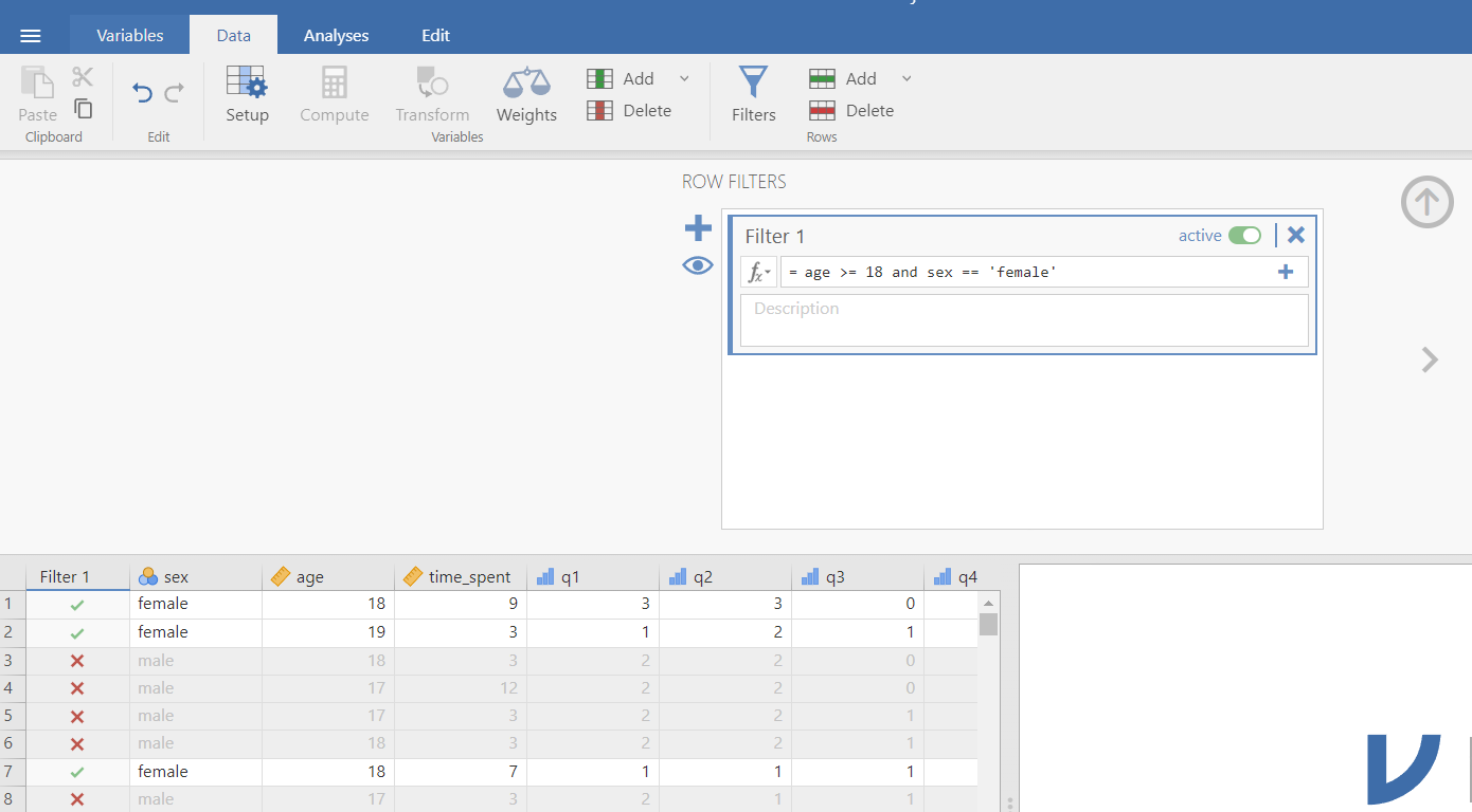
Figure 3.18: Combining conditions with “and” operator in one expression.

Note that in the above expression we can also use double quotes around the "female" (i.e., age >= 18 and sex == "female") or even the coded value (i.e., age >= 18 and sex == 2).

b) by adding the second condition (i.e. sex == "female") as another expression to “Filter 1” (by clicking the small + beside the first expression) (Figure 3.19):

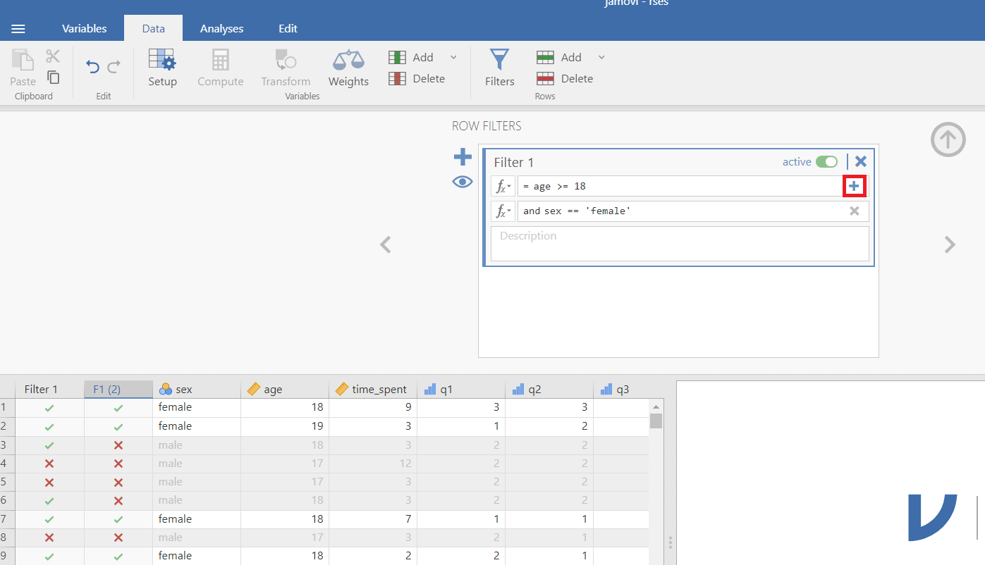
Figure 3.19: Multiple expressions in the same filter.

This additional expression comes to be represented with its own column F1(2) (Figure 3.19), and by looking at the ticks and crosses, we can see which expression is responsible for excluding each row.

c) adding a new “Filter 2” (by selecting the large + to the left of the filters dialog box) (Figure 3.20). In this case, we can activate or inactivate the filters separately.

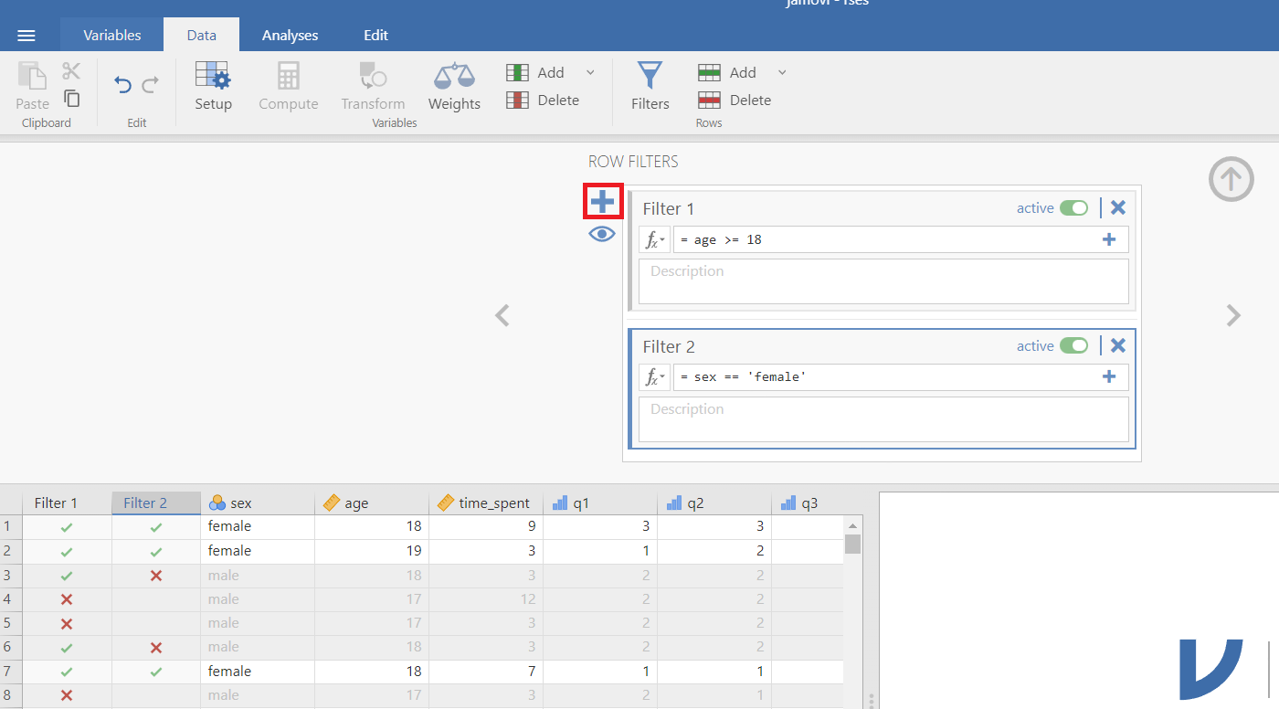
Figure 3.20: Multiple expressions using multiple filters.

We close the filter settings by pressing the arrow in the top-right corner .

Important

Filters in Jamovi exclude the rows for which the expression is not true. When filters are active, all results will be based on the filtered data. If we want to see unfiltered results we will either need to delete the filter or toggle it to inactive.

3.9 Transforming a variable

3.9.1 Transform a quantitative variable into a qualitative variable

Sometimes it can be useful to convert a quantitative variable into a qualitative variable with levels. For example, the time_spent can be categorized as follows:

less than or equal to 3 “0-3”
4 to 7 “4-7”
8 to 11 “8-11”
greater than 11 “>11”

Select time_spent variable and click the Transform button from the toolbar of the Data tab. This opens the “TRANSFORMED VARIABLE” view, where we can set the name of the transformed variable such as time_spent2 and create the transformation. To do this, select the source variable, the time_spent in this case, in the Source Variable field and create a new transformation using transform field (Figure 3.21), which is initially set to ‘none’.

Figure 3.21: Setting up a new transformation of a variable.

This opens the “TRANSFORM” view where Jamovi gives each transformation a name (e.g., Transform 1; if we want we can change it). This allows us to use it again later on other variables if we wish. We can also add a description (Figure 3.22).

Figure 3.22: Box for adding conditions to the transformation.

Now we need to add conditions. Jamovi uses simple if ... else statements and executes each statement starting from the top. So let’s start!

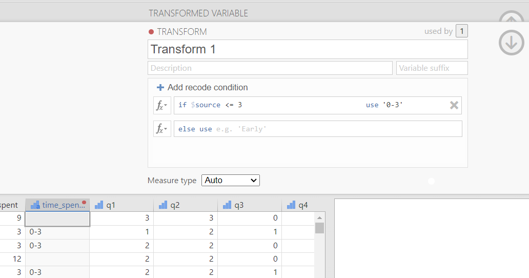
First, select + Add recode condition. Second, we need to fill the boxes with the information as follows (Figure 3.23):

The $source is the variable we want to transform (here time_spent)- don’t change this.
Select the appropriate comparison operator (here <= )
In the next box, we will put the time_spent value we want as the cut off point (e.g., 3).
After the use, add our new label (here '0-3'). If we are using text we must enclose it in '...'

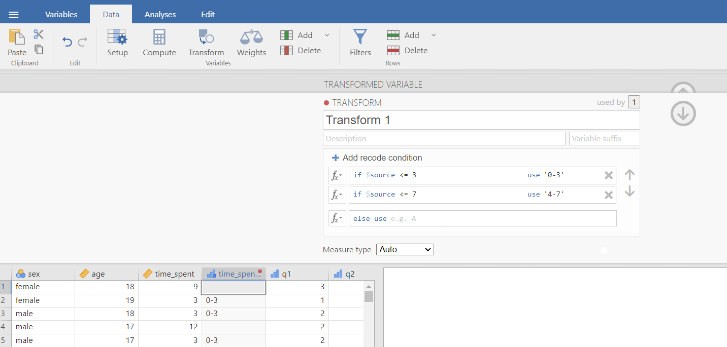
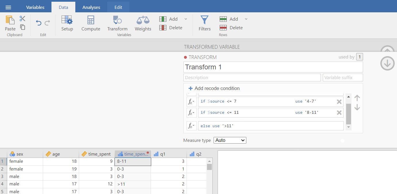
Figure 3.23: Adding the first condition (0-3).

We can add as many conditions as we want by selecting + Add recode condition. This will add a new if $source line into the box (Figure 3.24). Remember they will be executed in order.

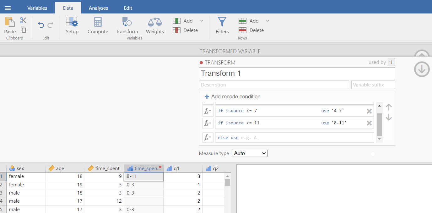
Figure 3.24: Adding the second condition (4-7).

Figure 3.25: Adding the third condition (8-11).

Finally, after the else use box just add the label for the data that does not meet the above conditions (here '>11'), as shown in Figure 3.26.

Figure 3.26: Adding the final label for the data that does not meet the above conditions (>11).

3.9.2 Reverse scoring of items

To compute the total score for all items of the RSES, we first need to reverse the scores of the negatively worded questions (3, 5, 8, 9, and 10). To do this, we can follow these simple steps.

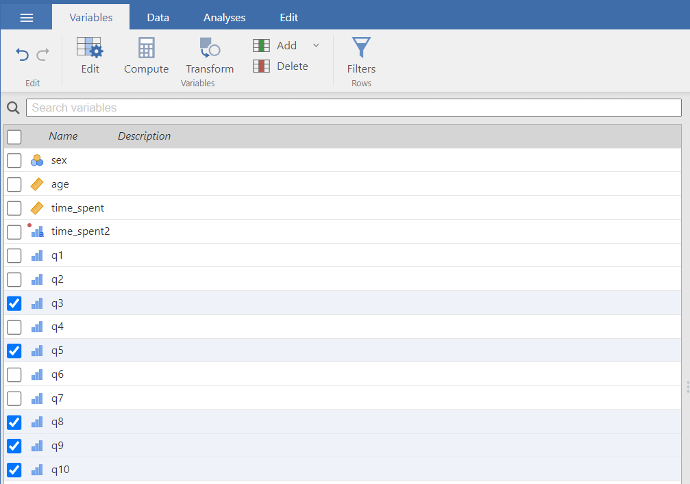
In the Variables tab, we select the checkboxes for the q3, q5, q8, q9, and q10 variables, as shown in Figure 3.27.

Figure 3.27: Select the variables to be reversed.

After that, we click on the Transform button ) from the toolbar of the Variables tab to open the Transform variable settings. Then, we Create New Transform, as shown in Figure 3.28.

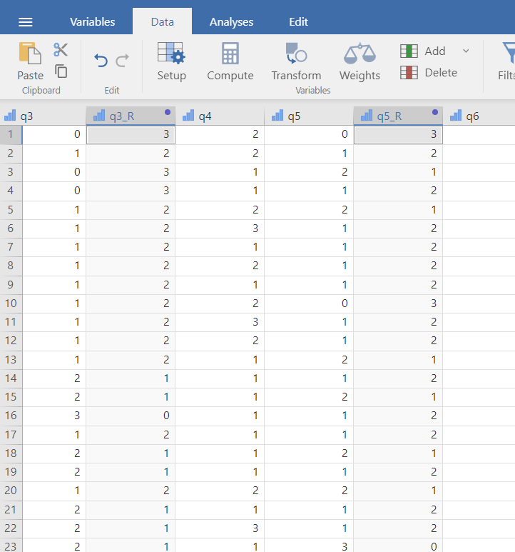
Figure 3.28: Open the Transform variable settings.

In the Transform view, we enter _R as a suffix for the variable names and specify 3-$source in the condition box, as shown in Figure 3.29.

Figure 3.29: Transform variable settings.

Figure 3.30: Data with the reversed variables.

3.10 Compute a new variable

Finally, we compute each participant’s total score (ranging from 0 to 30) based on their responses to the 10 questions of the Rosenberg Self-Esteem Scale.

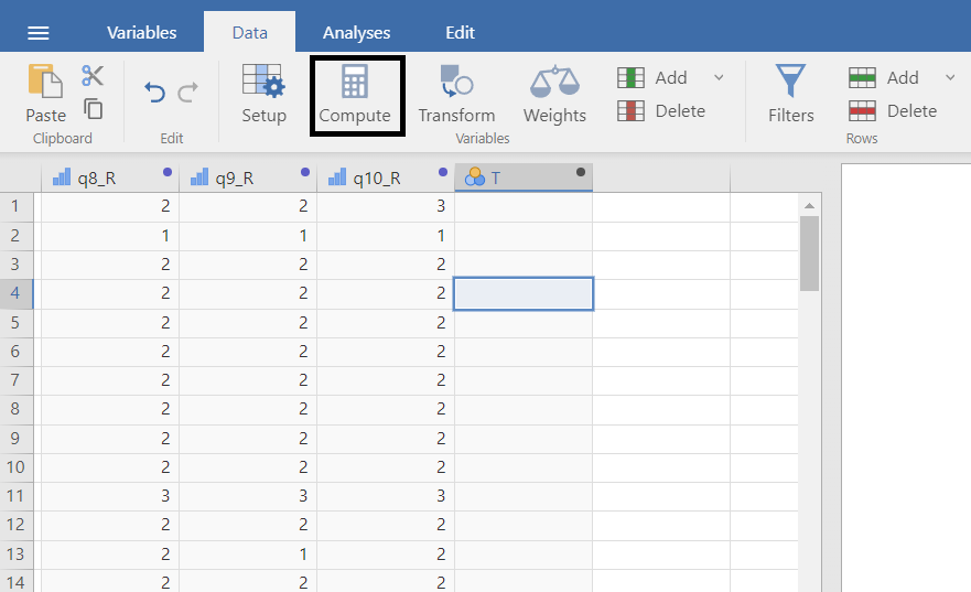
Adding computed variables to a Jamovi spreadsheet is straightforward. Click on the Compute button ) from the toolbar of the Data tab. An empty column has been created at the end of our dataset (Figure 3.31). The black dot symbol in the right of the column header indicates that this is a computed variable.

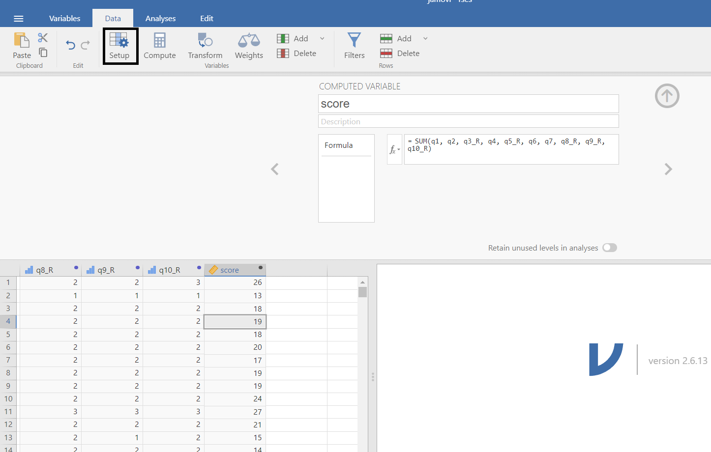
To set up the computed variable, either double-click the column header, or click the Setup button ) in the Data tab. This opens the “COMPUTED VARIABLE” view, where we can name the computed variable score. Next, we select the SUM function from the available options for use in the Formula box. Finally, we add the q-variables in the formula separated by comma (note that we must use the reversed variables in the sum) and we press ENTER (Figure 3.32).

Figure 3.32: Computation of the total score.