1 Introduction – Basic Statistics for the Social Sciences

1.1 Why learn basic statistics?

Knowledge of the fundamental principles of statistics, data analysis, and research methodology is essential for professionals in psychology and other social sciences today for three main reasons:

Understanding key statistical indicators: This knowledge allows professionals to interpret data and indicators from sources such as ELSTAT, EUROSTAT, and WHO. With this expertise, they can effectively assess and verify relevant information from around the world, hereby helping to counter misinformation. Key examples of these indicators include population health status, social inequalities, rates of violence and crime, unemployment rates, educational attainment levels, poverty rates, and access to healthcare services.
Critically analyzing research studies: Professionals are better equipped to evaluate research studies and their findings, ensuring they can identify strengths, weaknesses, and potential biases.
Conducting independent research: Familiarity with statistics enables professionals who conduct their own research to collaborate more effectively with statistical experts, enhancing the overall quality of their work.

1.2 The discipline of Statistics

The word “statistics” originates from the Latin “status”. Initially, it referred to the political state of a region, with “statista” used for recording information like censuses or data on a state’s wealth. Over time, the meaning and use of statistics broadened, and its scope evolved.

Today, Statistics is an applied mathematical science that, according to Croxton and Cowden, can be defined as “the science of collection, presentation, analysis, and interpretation of numerical data”.

Statistics includes different theoretical frameworks such as traditional (frequentist) statistics and Bayesian statistics. In this course, we will cover classical parametric and nonparametric statistical tests of traditional statistics.

Relying heavily on probability theory and empirical methods, statistics aims to describe and summarize data as well as to draw inferences about the population from which the data are derived. Therefore, the discipline of traditional (frequentist) statistics includes two main branches (Figure 1.1):

Descriptive statistics that includes measures of frequency and measures of location and dispersion. It also includes a description of the shape of the data distributions.
Inferential statistics that aims at generalizing conclusions made on a sample to a whole population. It includes estimation and hypothesis testing.

Figure 1.1: The discipline of statistics and its two branches, descriptive statistics and inferential statistics

In a research study, both descriptive and inferential statistics are commonly used. First, researchers present descriptive statistics (e.g., demographic data, baseline characteristics) to provide a clear snapshot of the sample. Then, inferential statistics are applied to test hypotheses and draw conclusions about the broader population from which the sample was drawn.

1.3 Talking about data

1.3.1 The “Age of data”

We are living in the “Age of Data”, where every day, an astonishing 2.5 quintillion ( $10^{18}$ ) bytes of data are generated worldwide. An example of how this era is transforming scientific research can be seen in large-scale multi-ancestry genome-wide association studies (GWAS), which are used to uncover the genetic basis of complex conditions like anxiety disorders. In a recent study, researchers analyzed genomic data from more than 1.2 million individuals across diverse populations, identifying more than 100 genes associated with stress and anxiety (Friligkou et al. 2024).

A second example is chatbots, which are designed to simulate conversations with users. ELIZA (1966) was one such program. Its famous “DOCTOR” script emulated a psychotherapist by rephrasing user statements as questions (Figure 1.2). Modern chatbots, such as ChatGPT, Gemini and Copilot, are large language models trained on vast amounts of text data (e.g., books, articles, websites, and user-generated content), hence the term “large”. Using deep learning techniques, these models aim to understand and generate human-like text, effectively responding to a wide range of user queries.

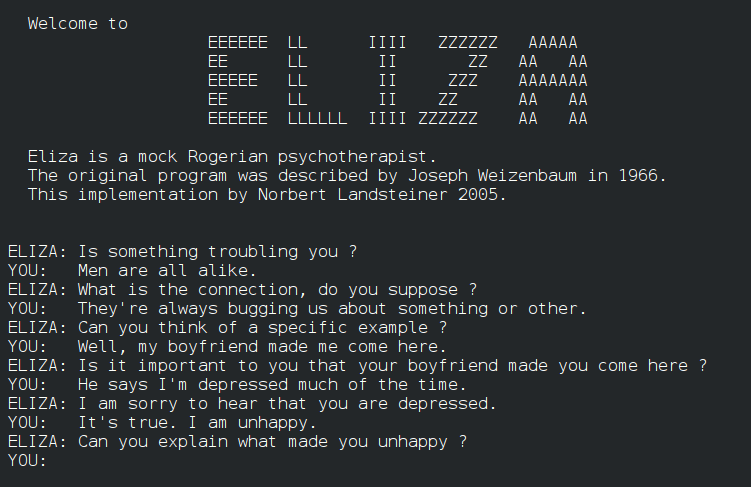
Figure 1.2: The most famous scenario simulated a psychotherapist of the Rogerian school.

Next is a YouTube video that explores the history of Eliza and chatbots.

1.3.2 Structure of data

There are three main data structures:

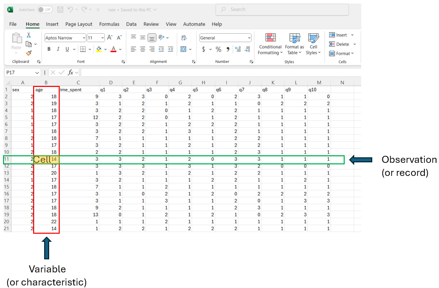
Structured data generally refer to highly organized tabular data, facilitating straightforward search, analysis, and processing. Examples include data stored in spreadsheets, such as Excel files, or in comma-separated values (CSV) files.
Semi-Structured data are a form of structured data that do not follow a strict tabular format but still have some organizational properties. For example, emails are semi-structured; they include fields like sender, recipient, subject, date, and time, and are also organized into folders such as Inbox, Sent, and Trash.
Unstructured data refer to information that lacks a predefined format or organization, such as open text (e.g., social media posts), images, videos, and other forms of multimedia.

In this course, we use data organized in a structured format, such as spreadsheets. Tabular data refer to data organized in a table with rows and columns (Figure 1.3). Each row represents an observation (or record), corresponding to a statistical unit in the dataset. The columns represent the variables (or characteristics) of interest. Cells are the individual units where rows and columns intersect. Each cell contains a data value corresponding to the observation for that row and the variable for that column.

Figure 1.3: A typical excel spreadsheet with row and columns.

1.3.4 From data to knowledge and decisions

Social, behavioral, and biomedical data can be transformed into information. This information can evolve into knowledge when social scientists and stakeholders interpret and understand it, allowing them to make informed decisions, shape policies, and implement interventions that address societal and health-related challenges more effectively (Figure 1.4).

Figure 1.4: From data to knowledge and action.

1.4 Social Statistics

Social statistics is a field of statistics applied in the social sciences to study social phenomena and trends. It employs various statistical methods of data collection, such as censuses, social surveys, and administrative records. These methods are commonly used by international organizations, government agencies, institutions, and researchers to analyze data related to social life, human behavior, and society as a whole.

The primary goal of social statistics is to provide objective, quantitative evidence that aids in understanding and interpreting social issues, ultimately informing the development of appropriate social policies.

Let’s explore some examples of official statistics from national governments and international organizations.

Example 1

Through its quarterly report Greece in Figures, the Hellenic Statistical Authority (ELSTAT) presents current and detailed statistical insights into Greece’s population, social structure, and economy.

An important socio-economic indicator at country level is the percentage of people at risk of poverty or social exclusion. Poverty and social exclusion severely disrupt the lives of those affected, perpetuating a cycle of disadvantage that can last for generations. This cycle not only limits personal growth but also poses significant challenges to social cohesion and economic stability within communities.

Figure 1.5: The percentage of people at risk of poverty or social exclusion in Eurozone. Greece (EL) is highlihgted.

In 2023, over a quarter (26.1%) of the Greek population was at risk of poverty or social exclusion, ranking Greece (EL) among the highest in the Eurozone, just behind Spain (ES; 26.5%), as shown in Figure 1.5.

Example 2

Gender inequalities and violence against women and girls are urgent social and public health issues that require immediate attention. A report, based on data from 2018 and published in May 2021, conducted by the World Health Organization, the London School of Hygiene and Tropical Medicine and the South African Medical Research Council, presents findings on the prevalence of violence against women.

The report found that the global lifetime prevalence of intimate partner violence among ever-partnered women was 30.0% (95% CI = 27.8% to 32.2%).

It is important to note that this estimated percentage (30%) is accompanied by a confidence interval (CI), which indicates a range from 27.8% to 32.2%. This interval reflects the precision of the estimate, and we will discuss it further in the subsequent sections of the course.

The report also mentioned that the prevalence of intimate partner violence among ever-partnered women was highest in the WHO African, Eastern Mediterranean and South-East Asia Regions with an estimated prevalence of approximately 37%. In contrast, the prevalence was lower in the high-income regions of America (23%) and the European and Western Pacific Regions (25%). This indicates that the prevalence of violence against women can differ significantly among regions, influenced by a range of socio-economic factors. In statistical terms, this suggests that there is a large variance in the data.

The report also references the Kiribati case; a country consisting of 33 islands situated in the central Pacific Ocean. The Kiribati family health study revealed an alarming prevalence of violence against women in Kiribati, with 68% of women aged 15–49 who had been in a relationship reporting experiences of violence (emotional, physical, and/or sexual) from a partner. This finding highlights how social statistics can assist in identifying rare cases (extreme values) to raise global concern and prompt immediate action.

The following YouTube video from UN Women is a campaign aimed at raising awareness about violence against women and girls.

1.5 Variables

1.5.1 Independent and dependent variables

A variable is a quantity or characteristic that is free to vary, or take on different values. Researchers design studies to test whether changes to one or more variables are associated with changes in another variable of interest.

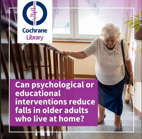
For example, if researchers hypothesize that a psychological intervention can help prevent falls in older adults living in the community more effectively than a standard approach, they could create a study to test this hypothesis. Participants would be randomly assigned to one of two groups: the experimental group, which receives the psychological intervention aimed at preventing falls, and the control group, which receives the usual care.

In this example, the type of intervention each participant received (i.e., the psychological intervention vs. usual care) is the independent variable (X), as it is the variable that the researchers manipulate. The dependent variable (Y), or the outcome variable, is the rate of falls over a time period, as it reflects the effect or outcome that the researchers measure to determine whether the intervention has an impact on reducing falls among older adults living in the community.

An independent variable (X) is the variable that is changed or controlled in a research study to examine its effect on another variable (Y), which represents the outcome being measured.

A dependent variable (Y) is the variable that is measured and assessed in a research study, influenced by the independent variables (Xs) being studied. It represents the outcome of the study.

It is important to note that we can construct both simple bivariate models and more complex, realistic multivariable models:

Diagram of a Bivariate Model (X → Y)

In this model, X is assumed to influence or predict Y. It’s commonly used to explore simple cause-and-effect associations or correlations, such as how a psychological intervention (X) might affect rate of falls in elderly (Y).

Diagram of Multivariable Model (X1, X2, X3 → Y)

This model allows for a more complex analysis, where several factors are considered simultaneously. For example, it can be used to study how a psychological intervention, gender, and balance (X1, X2, X3) together might affect rate of falls in elderly (Y), helping to capture the combined effects of multiple influences on the outcome.

1.5.2 Confounding variable

It is often essential to analyze the association between an independent variable (X) and a dependent variable (Y) while considering confounding variables, which should be controlled to prevent distortion of results.

A confounding variable is defined as one that is related with both the independent and the dependent variables and does not lie on the causal pathway between them.

For example, consider a study investigating the link between caffeine intake (X) and lung cancer (Y). Without accounting for confounding variables, such as smoking, the results may suggest a misleading association between caffeine and occurrence of lung cancer that is not truly causal.

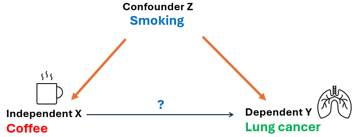
Smoking may be a potential confounding variable because it is:

related to caffeine consumption: Smokers often consume more caffeine (e.g., through coffee or energy drinks).
direct Cause of lung cancer: Smoking is a well-established cause of lung cancer and significantly increases the risk of developing the disease.
not directly part of the causal pathway: Smoking does not lie in the causal pathway between caffeine and lung cancer.

Comment

The causal pathway refers to the sequence of events or mechanisms through which an independent variable influences a dependent variable. It demonstrates how changes in the independent variable lead to changes in the dependent variable, often involving intermediary variables.

Confounding can be controlled either before or after a study is conducted. Various methods are available to control for confounding, including matching, stratification, and more advanced multivariate techniques (Grimes and Schulz 2002).

Pairwise matching: In a case-control study where smoking is considered a confounding variable, cases and controls can be matched based on smoking status.
Stratification: After a study is conducted, results can be stratified by levels of the confounding variable. In the smoking example, results would be calculated separately for smokers and non-smokers to determine if the same effect occurs independently of smoking.
Multivariate techniques: Mathematical modelling examines the potential effect of one variable while simultaneously controlling for the effect of many other variables.

1.6 Types of data in variables

Data in variables can be either categorical or numerical (otherwise known as qualitative and quantitative) in nature (Figure 1.7):

Figure 1.7: Broad classification of the different types of data with examples.

Note

The type of data in variables is an important factor in determining the most appropriate statistical analysis of the data.

1.6.1 Categorical data

A. Nominal data

Nominal data consists of distinct, unordered categories that are labeled but not measured, only counted. These categories can be binary, such as diagnosed/not diagnosed with depression, or they can have more than two categories, such as eye color (e.g., brown, blue, green, gray) or type of therapy (e.g., cognitive-behavioral therapy, psychoanalysis, humanistic therapy).

Numerical representation of categories are just codes

We can represent diagnosed/not diagnosed with depression as 1/0 and cognitive-behavioral therapy/psychoanalysis/humanistic therapy as 1/2/3 for therapy type. Unlike numerical data, the numbers assigned to categories do not have mathematical meaning; they are merely codes.

B. Ordinal data

When categories can be ordered, the data are of ordinal type. For example, patients may rate their pain as minimal, moderate, severe, or unbearable. In this case, there is a natural order to the values, as moderate pain is more intense than minimal but less than severe. Another common example of ordinal data is the Likert scale, where respondents might indicate their level of agreement with a statement on a scale such as from 1 (strongly disagree) to 5 (strongly agree).

IMPORTANT

Ordinal data are often transformed into binary data to simplify analysis, presentation, and interpretation, though this can result in a loss of information.
Although the Likert scale consists of ordered categories, the levels can be treated like numeric data, allowing scores from a questionnaire to be summed or averaged for a comprehensive assessment of respondents’ attitudes or feelings (total score of the participant).

1.6.2 Numerical data

A. Discrete data

Discrete data can take only a finite number of values (usually integers) in a range, for example, the number of children in a family or the number of days missed from work. Other examples are often counts per unit of time such as the number of visits to the psychotherapist in a year, or the number of epileptic seizures a patient has per month.

In practice discrete data are often treated in statistical analyses as if they were ordinal data. Although this approach may be acceptable, it may not fully optimize the use of our data.

B. Continuous data

Continuous data are numbers (usually with units) that can theoretically take any value within a given range. Examples of continuous variables include height, weight, body temperature, and reaction time. However, in practice, these variables are often measured discretely, constrained by the precision of measuring instruments and the study’s specific objectives. For instance, although height can be a continuous value, it is typically recorded in discrete steps. A person may measure 172.345 cm tall, but this would usually be recorded as 172 cm.

Categorization of numerical data leads to a loss of information

It is important to note that continuous data are often categorized to create categorical variables. For example, body mass index (BMI)—a continuous variable that measures weight relative to height—is typically converted into an ordinal variable with four categories: underweight, normal weight, overweight, and obese. However, dividing continuous variables into categories results in a considerable loss of information. Furthermore, the reverse transformation is impossible; a categorical variable cannot be transformed into a continuous variable.

Next is a YouTube video by Associate Professor Mike Marin from the University of British Columbia that comprehensively explains the different types of variables.