flowchart LR
  A(Analyses) -.-> B(Regression) -.-> C(Linear Regression)
8 LAB X: Simple linear regression
When we have finished this Lab, we should be able to:
In this Lab, we will use the “LungCapacity” dataset.
8.0.1 Opening the file
Open the dataset named “LungCapacity” from the file tab in the menu:
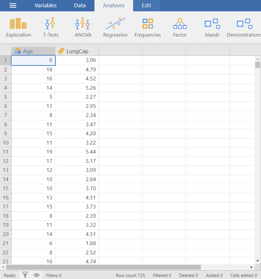
Double-click on the variable name Age and change the measure type from nominal ![]() to continuous
to continuous ![]() .
.
8.0.2 Research question
Let’s say that we want to model the association between age (in years) and lung capacity (in liters) for the sample of 725 participants in a survey. In other words, we want to find the parameters of a mathematical equation such as \(y = \alpha + \beta \cdot x\).
8.0.3 Hypothesis Testsing
8.0.4 Scatter plot
We start our analysis by creating the scatter plot of the response variable LungCap and the explanatory variable Age.
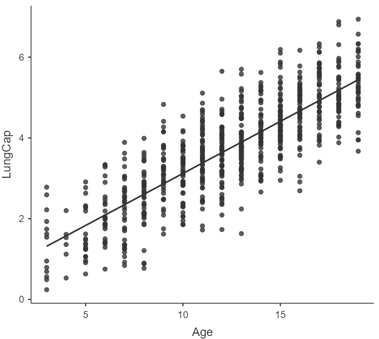
There is a clear upward trend indicating that increase in Age tends to coincide with increase in LungCap. Moreover, the trend seems to be linear, so a straight line can capture the overall pattern.
8.0.5 Linear regression
The process of fitting a linear regression model to the data involves finding a straight line that can be considered as the best representation of the overall association between age and lung capacity.
To choose a line, we need to explain what we mean by the “best representation” of the data. A “best-fitting” line refers to the line that minimizes the sum of squared residuals (RSS). Therefore, we refer to the resulting model as the least-squares linear regression model and to the corresponding line as the least-squares regression line.
8.0.6 Fit a simple linear regression model
On the Jamovi top menu navigate to
as shown below (Figure 8.3).
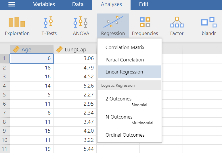
The Linear Regression dialogue box opens (Figure 8.4). From the left-hand pane drag the variable LunCap into the Dependent Variable field and the variable Age into the Covariates field on the right-hand side, as shown below:
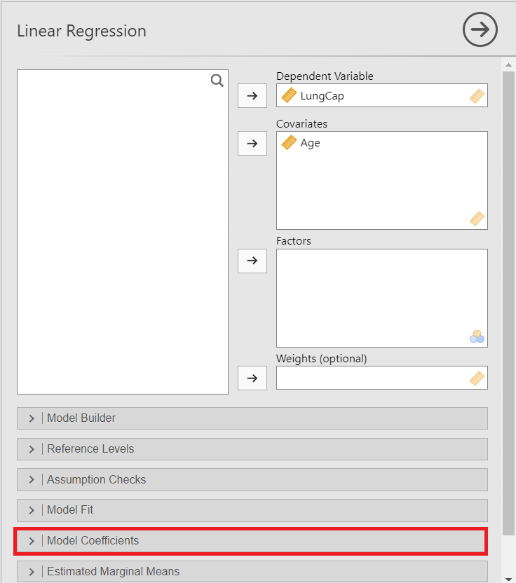
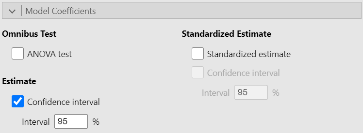
Additionally, from the Model Coefficients section tick the box “Confidence interval” in Estimate (Figure 8.5):
The output table with the model coefficients should look like the following (Figure 8.6):
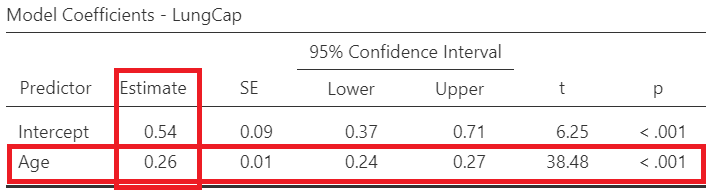
Now, let’s find the model equation from the regression table in Figure 8.6. In the Estimate column are the intercept \(a=0.54\) and the slope \(b=0.26\) for Age. Thus, the equation of the regression line becomes:
\[ \begin{aligned} \widehat{y} &= a + b \cdot x\\ \widehat{\text{LungCap}} &= a + b \cdot\text{Age}\\ \widehat{\text{LungCap}}&= 0.54 + 0.26\cdot\text{Age} \end{aligned} \]
Finally, the quality of our simple linear model is presented in Figure 8.7:
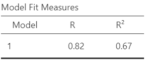
In our example takes the value 0.67. It indicates that about 67% of the variation in lung capacity can be explained by the variation of the age. In simple linear regression \(\sqrt{0.67} = 0.82\) which equals to the Pearson’s correlation coefficient, r.